library(tidymodels)
library(tidyverse)
library(palmerpenguins)This session was recorded and uploaded on YouTube here:
In this session, we will learn how to use the {recipes} package to transform data for statistical modeling. {recipes} is a powerful tool for pre-processing data in a tidy and reproducible way. This package is an integral part of the the {tidymodels} workflow, which provides a unified framework for building and evaluating statistical models. For more information regarding the {recipes} package, please visit the recipes webpage
Why do we need to pre-process data?
Well, it’s all about setting the stage for statistical tests!
Data pre-processing is the process of transforming raw data into a format that is suitable for statistical modeling. Each statistical test has its unique assumptions, so sometimes we need to fine-tune our data to meet those criteria. These transformations are tailored to the specific statistical test at hand. Pre-processing may include:
Cleaning the data: This can include removing missing values or outliers.
Transforming the data: This may involve converting variable to different scales, creating new variables, or combining existing variables. An example of this can be logarithmic transformation.
Normalizing the data: This involves scaling the variables to have a similar mean and variance.
In today’s session we’ll focus on two fundamental pre-processing techniques: transformations and normalizations! Keep in mind that the transformations you choose will be determined by both the statistical test you are performing and your research question. It’s also essential to run some basic checks to ensure your data aligns with the assumptions of your chosen test.
Pre-processing data with recipes
The {recipes} package provides a simple and efficient way to pre-process data for statistical modeling. It works by creating a recipe, which is a sequence of pre-processing steps that are applied to the data, right before it enters statistical modelling.
To create a recipe, we use the recipe() function. This function requires a formula as input. This formula will specify the dependent variable (outcome) and the independent variables(predictors) in the model. We also require data frame with the raw data.
Once we have created a recipe, we can apply it to the data using the prep() function. This function takes the recipe and the data frame as input and returns a pre-processed data frame. The bake() function takes a new data frame as input (such as, the test data set if data split was performed) and also returns a pre-processed data frame.
Example
Let’s use the {recipes} package to pre-process the penguins data set from the {palmerpenguins} package.
Let’s first take a quick look into the data!
# Load the penguins dataset
penguins %>%
  glimpse()
Rows: 344
Columns: 8
$ species <fct> Adelie, Adelie, Adelie, Adelie, Adelie, Adelie, Adel…
$ island <fct> Torgersen, Torgersen, Torgersen, Torgersen, Torgerse…
$ bill_length_mm <dbl> 39.1, 39.5, 40.3, NA, 36.7, 39.3, 38.9, 39.2, 34.1, …
$ bill_depth_mm <dbl> 18.7, 17.4, 18.0, NA, 19.3, 20.6, 17.8, 19.6, 18.1, …
$ flipper_length_mm <int> 181, 186, 195, NA, 193, 190, 181, 195, 193, 190, 186…
$ body_mass_g <int> 3750, 3800, 3250, NA, 3450, 3650, 3625, 4675, 3475, …
$ sex <fct> male, female, female, NA, female, male, female, male…
$ year <int> 2007, 2007, 2007, 2007, 2007, 2007, 2007, 2007, 2007…Before we dive into data transformations, it is essential to have a clear research question in mind. Remember the data transformations depends on the research question.
In this case, our research question is:
Given knowledge of body mass, species, and sex, can we accurately estimate bill depth in penguins?

Given our research question, we will fit a simple linear regression model using the lm() function in R. Then, we will use the tidy() function to view the output of the model.
The tidy() function constructs a tibble that summarizes the model’s statistical findings. This includes estimates (aka. as coefficients) and p-values. For more information about the tidy function consult its documentation webpage.
# Let's define our model
test_model <- lm(bill_depth_mm ~ body_mass_g + species + sex, data = penguins)
# Let's take a look into the output of our model
tidy(test_model)
# A tibble: 5 × 5
term estimate std.error statistic p.value
<chr> <dbl> <dbl> <dbl> <dbl>
1 (Intercept) 15.2 0.479 31.8 3.34e-102
2 body_mass_g 0.000706 0.000140 5.05 7.48e- 7
3 speciesChinstrap 0.0543 0.118 0.460 6.46e- 1
4 speciesGentoo -4.34 0.217 -20.0 7.53e- 59
5 sexmale 1.03 0.128 8.05 1.52e- 14The previous model estimates the bill depth based on body mass, species and sex. The p-values for body mass, species, and sex are significant, but the estimates appear to be very small. This can indicate that the relationships between the variables are statistically significant, but they are weak.
An interpretation of the results can be as follows: If we keep all other variables constant (i.e species and sex), a one-unit increase in body mass is associated with a very small increase (0.000706 mm) in bill depth.
Verifying the assumptions of a linear regression model
Linear regression models require certain assumptions to be met in order to be valid. These assumptions include:
Linearity: The relationship between the dependent variable and the independent variables is linear.
Normality: The residuals of the model are normally distributed. The residuals of a model are the differences between the observed values and the predicted values of the dependent variables.
Homoscedasticity: The variance of the residuals is constant across all values of the independent variables
We can use residual plots to check whether our model meets these assumptions.
One of the easiest residual plots to interpret is the Q-Q plot of the residuals. In a Q-Q plot, the residuals of the model are plotted against the theoretical quantiles of the normal distribution. If the residuals are normally distributed, the points in the Q-Q plot will fall along a straight line.
Let’s check if our model meets those assumptions using the plot() function. The function plot() will generate several plots to check your model assumptions. Here we only want the Q-Q plot of the residuals of the model, which we get by using the argument which = 2.
# Check linear model assumptions
plot(test_model, which = 2)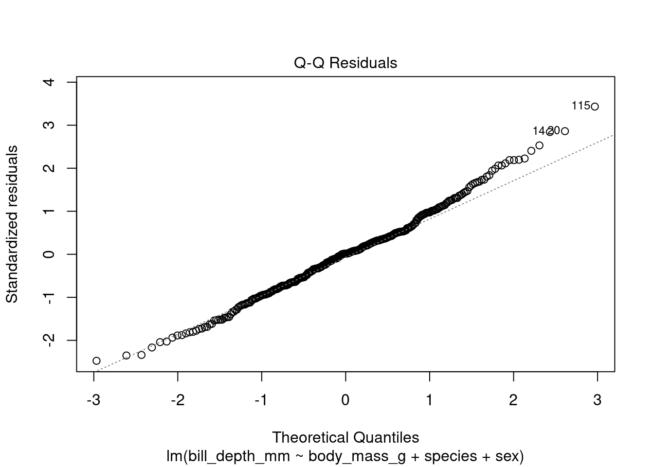
The resulting Q-Q plot shows that the residuals of the model are not normally distributed, as the points in the plot do not fall along a straight line (they are deviating in the upward part of the plot). This suggests that we may need to transform the data before fitting the linear regression model.
If the Q-Q plot of the residuals deviates upwards, it means that there are more outliers in the upper tail of the distribution than in the lower tail. This can be caused by a number of factors including a bimodal distribution of the dependent variable (i.e bill depth). If the dependent variable has a bimodal distribution, the residuals will also have a bimodal distribution. This is because the linear regression model will try to fit a straight line through the center of the distribution, which will result in errors for the outliers in the upper and lower tails.
Based on this, let’s make a histogram to investigate the distribution of bill depth! We will use the ggplot() function for this.
ggplot(penguins, aes(x = bill_depth_mm)) +
  geom_histogram()
`stat_bin()` using `bins = 30`. Pick better value with `binwidth`.Warning: Removed 2 rows containing non-finite outside the scale range
(`stat_bin()`).
The histogram shows that the distribution of bill depth appears to be bimodal. This suggests that the Q-Q plot is deviating upwards because of the bimodal distribution of bill depth.
To address this issue, we can transform the bill depth variable using a log transformation. After transforming the bill depth variable, we can generate a new Q-Q plot of the residuals. The new Q-Q plot shows that the residuals should now be normally distributed.
Creating a recipe for Data transformation
Based on the previous, we will now create a recipe to transform our data. This will helps us to improve the normality of the residuals and make data more interpretable.
To create a recipe we will perform the following steps:
Step 1: Specify the model
We first need to specify the model to the recipe. We do this using the recipe() function. In this case, we will use the same model as we did before. The bill depth (bill_depth_mm) is our outcome variable (y), and the body mass (body_mass_g), species (species), and sex (sex) are our predictors/exposures.
Step 2: Specify the data transformations
Next, we need to specify the data transformations that we want to perform. Every data transformation starts with step_. A complete list of all the possible transformations that you can perform using the recipes package can be consulted in the recipes reference section.
In this example, we will perform a logarithmic transformation using step_log(). This will help us improve the normality of the residuals. We also want to perform a normalization using step_normalize(). This will make the data more interpretable by setting the mean of the predictors to zero.
Normalization is a data transformation technique that sets the mean of a variable to zero and the standard deviation to one. This can be useful for improving the interpretability of the data, especially when using linear regression models.
For example, let’s say we have a linear regression model that predicts bill depth based on body mass. If we do not normalize the data, the intercept of the model will represent the bill depth when the body mass is zero. However, this is not a very meaningful value, since penguins do not have zero body mass.
After normalizing the data, the intercept of the model will represent the bill depth when the body mass is at the mean value. This is a much more meaningful value, as it represents the average bill depth of penguins.
In every transformation using step_, you always need to specify what you want to transform. In this case we wanted to log transform all numeric variables. For this we used step_log(all_double()). For normalization we used use use step_normalize (all numeric_predictors()) This specification will indicate the recipe to only normalize body mass (body_mass_g), since it is the only numeric predictor.
Step 3: Prepare and bake the data
Finally, we need to prepare and bake the data using the prep() and bake() functions. As mentioned before, this steps are really useful when creating recipe outside the {tidymodels} workflow and also when data splitting has been performed.
Prepping the data will perform all the calculations for the data transformations in the training data set. Baking the data will perform the data transformations on the test or validation set.
In this example, we did not perform data splitting, so we will set bake(new_data=NULL)
transformed_penguins <- penguins %>%
  # Step 1: specify the model
  recipe(bill_depth_mm ~ body_mass_g + species + sex) %>%
  # Step 2: specify data transformations
  step_log(all_double()) %>%
  # Step 2: specify data transformations
  step_normalize(all_numeric_predictors()) %>%
  # Step 3: prepare data
  prep() %>%
  # Step 3: bake the data
  bake(new_data = NULL)

transformed_penguins
# A tibble: 344 × 4
body_mass_g species sex bill_depth_mm
<dbl> <fct> <fct> <dbl>
1 -0.563 Adelie male 2.93
2 -0.501 Adelie female 2.86
3 -1.19 Adelie female 2.89
4 NA Adelie <NA> NA
5 -0.937 Adelie female 2.96
6 -0.688 Adelie male 3.03
7 -0.719 Adelie female 2.88
8 0.590 Adelie male 2.98
9 -0.906 Adelie <NA> 2.90
10 0.0602 Adelie <NA> 3.01
# ℹ 334 more rowsThe variable transformed_penguins will contain the pre-processed (transformed) data, which is ready for statistical analysis.
We can now re-run our linear model using the pre-processed data. To do this, we will simply replace the data argument to include the transformed_penguins data. e will call this the transformed_model and we will use tidy() to look at the output of the model. We will also use plot() to check linear assumptions.
# Fit linear model on transformed data
transformed_model <- lm(bill_depth_mm ~ body_mass_g + species + sex, data = transformed_penguins)
# Look at the output of the model
tidy(transformed_model)
# A tibble: 5 × 5
term estimate std.error statistic p.value
<chr> <dbl> <dbl> <dbl> <dbl>
1 (Intercept) 2.90 0.00799 363. 0
2 body_mass_g 0.0346 0.00637 5.44 1.05e- 7
3 speciesChinstrap 0.00312 0.00670 0.466 6.41e- 1
4 speciesGentoo -0.262 0.0123 -21.3 7.56e-64
5 sexmale 0.0596 0.00729 8.18 6.52e-15# Check linear assumptions
plot(transformed_model, which = 2)
As we observe, the new Q-Q plot shows that the residuals are now normally distributed (after log transformation).
When we log transform the outcome variable in a linear regression model, the coefficients of the model represent the percentage change in the outcome variable for a one unit increase in the predictor variable, assuming that all other predictor variables are held constant.
For example, in the example we have been discussing, the coefficient for the body_mass_g variable is 0.03463. This means that a one unit increase in body mass will lead to a 3.463% increase in bill length, assuming that the species and sex of the penguin are held constant.
It is important to note that the interpretation of the coefficients of a linear model changes after a log transformation. Before the log transformation, the coefficients represented the change in the outcome variable for a one unit increase in the predictor variable, measured in the original units. After the log transformation, the coefficients represent the percentage change in the outcome variable for a one unit increase in the predictor variable, measured in standard deviations.
Now, let’s try pre-processing our data in a different ways!
We will now log transform all outcome variables using step_log (all_outcomes()) . We will also remove highly correlated variables using step_corr(all_numeric_predictors()),and we will remove variables with non-zero variance usingstep_nzv(all_numeric-predictors()).
transformed_penguins <- penguins %>%
  recipe(bill_depth_mm ~ body_mass_g + species + sex) %>%
  step_log(all_outcomes()) %>%
  step_normalize(all_numeric_predictors()) %>%
  step_corr(all_numeric_predictors()) %>%
  step_nzv(all_numeric_predictors()) %>%
  prep() %>%
  bake(new_data = NULL)
Keep in mind that the order in which you perform the pre-processing steps matters!!!
The recommended pre-processing ordering, taken from the {recipes} website, is as follows:
- Impute
- Handle factor levels
- Individual transformations for skewness and other issues
- Discretize (if needed and if you have no other choice)
- Create dummy variables
- Create interactions
- Normalization steps (center, scale, range, etc)
- Multivariate transformation (e.g. PCA, spatial sign, etc)
For more information regarding the order in which the pre-processing steps should be performed visit the articles section in the recipe package Ordering of Steps.
Done!