R Coding Club - Debugging in R

This session was recorded and uploaded on YouTube here:

Debugging is a very broad topic, encompassing a wide array of scenarios that are often highly context-specific. We can encounter diverse challenges that need to adopt different debugging methods depending on the problems we encounter.

Here we illustrate some of the fundamental steps to understanding bugs and address some of the most common debugging strategies.

Error messages

The initial step in debugging is to understand the error message. Error messages are often quite explicit, offering hints of the type of errors, locations, and suggestions to fix the issues. But they sometimes can be too specific and get too technical so that it is hard to understand what they mean.

Don’t be alarmed by error messages! Encountering them is very common and a regular part of the process no matter your skill level. Getting used to the presence of error messages and learning to read them is essential. Indeed, the very first step of debugging is to read the error message. Let’s begin with a straightforward example:

sum(c("a","b"))

Error in sum(c("a", "b")): invalid 'type' (character) of argument

The c() function aggregates elements into a vector and the sum() function computes the total from a vector of numeric values. As we can’t calculate the sum of letters, this leads to an issue. The prompted error message provides a clue saying this is an invalid “type” assertion, suggesting a character input.

Reread your code

The second step of debugging involves rereading your code when encountering an error.

In many instances, a significant part of the issues we face during coding is overlooking a comma, a bracket, a quote, or other typo. In the code below as an example, we forgot a comma. Unfortunately, the error message is not very helpful in this case:

paste("Hi!" "what's up?")

Error: <text>:1:13: unexpected string constant
1: paste("Hi!" "what's up?"
                ^

This is why it is important to read over the code again if you don’t understand the error message.

Function documentation

In the previous example, if we understand the functionality of the paste() function, we can identify the source of the error.

We can access the function documentation (see image below) by either clicking on the function name and pressing F1, or by typing ?paste or help(paste) directly into the console.

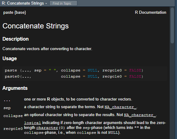
Documentation for the `paste()` function.

Namespace issues

Namespace is the term used to describe what functions are exposed to users inside a package. So the namespace of the package, for instance, {dplyr}, includes the functions select(), filter(), or mutate(). The functions and objects available in a package’s namespace can be found by using the :: before the package name and hitting Tab to see a list of objects (e.g. dplyr::).

Namespace issues occur when we want to use a function from a specific package, but we’re actually using a function from a different package. For instance, consider the case of attempting to filter values within the CO2 dataset. We might assume we are using the filter() function from the {dplyr} package, so we run this:

library(magrittr)
CO2 %>% 
  filter(uptake > 30)

Error: object 'uptake' not found

But we get an error, indicating that the “uptake” object cannot be found. Why is that the case? From a programming perspective, it’s possible for multiple functions with the same name to coexist, and when loading them collectively, certain function names may get overridden. In this particular case, we wanted to use the filter()function from the {dplyr} package but instead are using the filter()function from the {stats} package. We can verify this checking the function documentation (by placing the cursor on the filter()function and pressing F1), as seen in the image below.

Checking the `filter()` function from the stats packages.

This can frequently occur when you have multiple packages loaded, and you may not always ensure that the functions are being overwritten or not. This is much more likely to happen when you load a lot of packages and don’t check to make sure that the functions you are using are overwritten or not.

When we load the {dplyr} package and then use the filter()function, it finally works:

library(dplyr)
CO2 %>% 
  filter(uptake > 30)

# A tibble: 40 × 5
   Plant Type   Treatment   conc uptake
   <ord> <fct>  <fct>      <dbl>  <dbl>
 1 Qn1   Quebec nonchilled   175   30.4
 2 Qn1   Quebec nonchilled   250   34.8
 3 Qn1   Quebec nonchilled   350   37.2
 4 Qn1   Quebec nonchilled   500   35.3
 5 Qn1   Quebec nonchilled   675   39.2
 6 Qn1   Quebec nonchilled  1000   39.7
 7 Qn2   Quebec nonchilled   250   37.1
 8 Qn2   Quebec nonchilled   350   41.8
 9 Qn2   Quebec nonchilled   500   40.6
10 Qn2   Quebec nonchilled   675   41.4
# ℹ 30 more rows

How to prevent Namespace issues?

The following function can be used as a tool to find conflicts with any function from all the packages you have loaded in your session:

conflicted::conflict_scout()

2 conflicts

• `filter()`: dplyr and stats

• `lag()`: dplyr and stats

Thanks to this function we can visualize that there are two possible conflicts with the filter()and lag() functions, which exist in both packages {dplyr} and {stats}.

Another good practice is to specify the packages in the functions like follows:

stats::filter()

In the previous case, we specify that we want to use the filter function in the {stats} package.

Reload, reinstall packages, and start R session

The following error informs us that one the packages is needing a higher version of another package than the one is currently loaded:

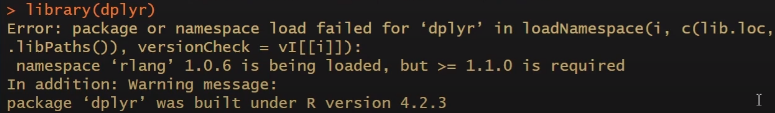
To solve this issue, you can try to:

Re-nstall packages. The following code string will force the re-installation of packages:
```
install.packages("rlang", force = TRUE)
```
Load the packages one by one.
Restart the R session if all the packages are correctly installed and loaded (image below).

Debug functions

In this section we cover the functions debugonce() and browser().

The function debugonce() allows us to set a one-time breakpoint in our code. When entering debugonce(function_name), it modifies the function so that when we run the function next, it causes it to enter into debugging mode. This allows us to interactively debug and inspect the function. Let’s explore an example involving a custom filtering function that contains an issue:

subset_co2 <- function(filter_condition) {
  dplyr::filter(CO2, filter_condition)
}
subset_co2(uptake > 35)

Error in `dplyr::filter()`:
ℹ In argument: `filter_condition`.
Caused by error:
! object 'uptake' not found

As we see from the error message, the problem seems to be that the object uptake is not found, even though we know that if we used that same code while using filter(), it would work. We can run debugonce() on the function and it will enter debug mode:

debugonce(subset_co2)
subset_co2(uptake > 35)

This mode is shown in the image below. Using the “next”, “continue”, and “stop” buttons that are found just above the RStudio Console, we can sequentially navigate line by line through your function and check the objects in our environment (the A section of the image).

A similar function is the browser(). This function will cause the function to enter the debug state at the line it is included in. So, you can place it where you think your problem is and start debugging from there. We run the following code:

subset_co2 <- function(filter_condition) {
  browser()
  dplyr::filter(CO2, filter_condition)
}
subset_co2(uptake > 35)

We re-enter the debugging state again. If we type out filter_condition into the Console (the B panel in the image), we see that it is not properly entering into the function. So the problem doesn’t come from within the function itself, the issue lies in the code outside the function.

R is a programming language created for data analysis and statistics rather than computer science. Non-standard evaluation refers to the code that is evaluated dynamically by expressions rather than by its value, allowing flexibility and a dynamic behavior. It is really useful when you are writing statistical code, but it can potentially introduce a cascade of errors when used in situations that require standard evaluation in the code strings.

Non-standard evaluation can be better explained by code that is quoted or unquoted. A very common example is when you use library():

# Non-standard evaluation
library(dplyr)

# Standard evaluation
library("dplyr")

The function library() uses both standard and non-standard evaluation here. It’s called non-standard because normally when code is unquoted like with dplyr, programming languages evaluate it by running it. But we know that dplyr isn’t actually an object in R so can’t run:

dplyr

Error in eval(expr, envir, enclos): object 'dplyr' not found

But when quoted:

"dplyr"

[1] "dplyr"

It gives us a character value back. R in general but especially {tidyverse} use non-standard evaluation frequently, since it makes coding and reading code easier, but makes errors and programming a bit more difficult.

So with our filtering condition (uptake > 30), we assumed we were using non-standard evaluation. But only some functions are designed for that, and our custom function is not designed to use it. So when we run it, R looks for the object uptake, but it doesn’t exist. It is a column in the dataset, but not an object in R.

Thankfully, {tidyverse} provides a method to easily use non-standard evaluation within custom functions. This method is called curly-curly ({ }), which we can use within the filter() function in our custom function (see in panel C of the image). This revised code below will work without issues.

subset_co2 <- function(filter_condition) {
  dplyr::filter(CO2, {{ filter_condition }})
}
subset_co2(uptake > 35)

# A tibble: 25 × 5
   Plant Type   Treatment   conc uptake
   <ord> <fct>  <fct>      <dbl>  <dbl>
 1 Qn1   Quebec nonchilled   350   37.2
 2 Qn1   Quebec nonchilled   500   35.3
 3 Qn1   Quebec nonchilled   675   39.2
 4 Qn1   Quebec nonchilled  1000   39.7
 5 Qn2   Quebec nonchilled   250   37.1
 6 Qn2   Quebec nonchilled   350   41.8
 7 Qn2   Quebec nonchilled   500   40.6
 8 Qn2   Quebec nonchilled   675   41.4
 9 Qn2   Quebec nonchilled  1000   44.3
10 Qn3   Quebec nonchilled   250   40.3
# ℹ 15 more rows